> For the complete documentation index, see [llms.txt](https://jheck.gitbook.io/hadoop/llms.txt). Markdown versions of documentation pages are available by appending `.md` to page URLs; this page is available as [Markdown](https://jheck.gitbook.io/hadoop/data-storage.md).
# Data storage
## Introduction to Databases
A database is a collection of data stored in some organized fashion.
The database software is the called the Database Management System (DBMS). For relational databases, it is called RDBMS. The database is the container created and manipulated via the DBMS.
#### Tables
Within a database, a table is a structured list of data of a specific type.
Usually with relational databases, the data stored in a table is one type of data or one list (e.g. one table for Customers, one table for Orders, etc.). Every table in a database has a name that identifies it. That name is always unique, meaning no other table in that database can have the same name.
Table have characteristics and properties that define how and what kind of data is stored in them. This set of information that describes a table is known as a **schema**. Schema are used to describe specific tables within a database.
#### Columns and Datatypes
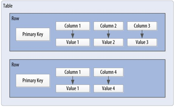
Tables are made up of columns.
A column contains a particular piece of information within a table. A column is a single field in a table. All tables are made up of one or more columns. Each column in a database has an associated datatype. A datatype defines what type of data the column can contain (e.g. Integer, Character Array, etc.).
Datatypes restrict the type of data that can be stored in a column (e.g. preventing the entry of alphabetical characters into a numeric field). Datatypes help sort data correctly and play an important role in optimizing the disk usage.
#### Rows and Primary Keys
Data in a table is stored in rows; each record saved is stored in its own row. A row is basically a record. Every row in a table should have some column (or set of columns) that uniquely identifies it (but this is not mandatory). This column (or set of columns) that uniquely identifies each row in a table is called a **Primary Key**.
The primary key meets the following conditions:
* No two rows can have the same unique primary key value.
* Every row must have a primary key value (NULL are not allowed).
* Values in the primary key columns should never be modified or updated.
#### Transactions
RDBMSs and SQL also support transactions. A key feature of transactions is that they execute virtually at first, allowing the programmer to undo (using rollback) any changes that may have gone awry during execution; if all has gone well, the transaction can be reliably committed.
A transaction is “a transformation of state” that has the **ACID**properties.
#### ACID Properties
ACID is an acronym for **Atomic**, **Consistent**, **Isolated**, **Durable**, which are the gauges we can use to assess that a transaction has executed properly and that it was successful.
**Atomic** means “all or nothing”; that is, when a statement is executed, every update within the transaction must succeed in order to be called successful.
**Consistent** means that data moves from one correct state to another correct state, with no possibility that readers could view different values that don’t make sense together.
**Isolated** means that transactions executing concurrently will not become entangled with each other; they each execute in their own space. That is, if two different transactions attempt to modify the same data at the same time, then one of them will have to wait for the other to complete.
**Durable**: once a transaction has succeeded, the changes will not be lost. This doesn’t imply another transaction won’t later modify the same data; it just means that writers can be confident that the changes are available for the next transaction to work with as necessary.
#### Schema
A database schema
* is the skeleton structure that represents the logical view of the entire database.
* defines how the data is organized and how the relations among them are associated.
* formulates all the constraints that are to be applied on the data.
* defines its entities and the relationship among them.
* contains a descriptive detail of the database.
### Bigtable: Genesis of NoSQL
In 2006, Google released a whitepaper that would outline a new paradigm for databases and data storage: **“Bigtable: A Distributed Storage System for Structured Data.”**
Bigtable was the distributed storage system for managing structured data at Google. However, unlike existing RDBMS platforms, Bigtable was designed to reliably scale to petabytes of data and thousands of machines to meet Google’s application workload demand.
Bigtable paved the way for several Apache projects, including HBase, Cassandra, MongoDB and others.
NoSQL, which stands for Not Only SQL, is an integral product of the big data movement, and the Google Bigtable paper was a major catalyst for the movement.
### Characteristics of NoSQL systems
**NoSQL DB are schemaless at design time and “schema-on-read” at runtime** - This means they do not have predefined columns, but columns are created with each PUT (INSERT) operation, and each record, document, or data instance can have a different schema from the previous instance.
**Data has no predefined relationship to any other object** - This means there is no concept of foreign keys or referential integrity, declarative or otherwise. Relationships may exist between data objects or instances, but they are discovered or leveraged at runtime rather than prescribed at design time.
**Joins are typically avoided** - In most NoSQL implementations, joins are kept to an absolute minimum, if not avoided altogether. This is typically accomplished by denormalizing data, often with a trade-off of storing duplicate data.
NoSQL systems are typically distributed (like Apache Cassandra or HBase) and are designed for fast lookups.
Write operations are typically faster as well, as many of the overheads of traditional relational database systems are not used, like datatype or domain checks, atomic/blocking transactions, or management of transaction isolation levels.
NoSQL systems, in the majority of cases, are built for scale and scalability from petabytes of storage to queries bounded in terabytes, performance, and low friction (having the ability to adapt to changes).
### Types of NoSQL systems
NoSQL systems come in several variants or categories:
**Key value stores** contain a set or sets of indexed keys and associated values. Values are typically uninterpreted byte arrays, but can represent complex objects such as nested maps, structs, or lists. The schema is not defined at design time. Examples of key value stores include Redis and Memcached.
**Column stores** or wide-column stores, which store data tables as columns rather than rows and have an ability to hold very large numbers of dynamic columns. Examples of Column stores include HBase, BigTable.
**Document stores** or document databases store documents, complex objects, such as JSON or BSON objects, or other complex, nested objects. The documents are assigned a key or document ID, and the contents would be the semi-structured document data. Examples of document stores include MongoDB and CouchDB .
**Graph stores** represent data in graph structures as nodes and edges, which are relationships between nodes. Examples of graph stores include Neo4J and GraphBase.
### NoSQL databases and CAP theorem
The **CAP theorem** is sometimes called Brewer’s theorem after its author, Eric Brewer.
The theorem states that within a large-scale distributed data system, there are three requirements that have a relationship of sliding dependency:
* **Consistency**: All database clients will read the same value for the same query, even given concurrent updates.
* **Availability**: All database clients will always be able to read and write data.
* **Partition tolerance**: The database can be split into multiple machines; it can continue functioning in the face of network segmentation breaks.
Brewer’s theorem is that in any given system, you can strongly support only two of the three. We have to choose between them because of this sliding mutual dependency.
In distributed systems, it is very likely that you will have network partitioning, and that at some point, machines will fail and cause others to become unreachable. Distributed systems need Partition Tolerance!
For NoSQL databases, it leaves with only two real options to compromise on: availability and consistency.


## Introduction to SQL
SQL is an abbreviation for **Structured Query Language**.
SQL is a language designed specifically for communicating with databases.
SQL is designed to provide the programmer with a simple and efficient way to read and write data from a database.
SQL has several advantages:
* SQL is not a proprietary language used by specific database vendors. Almost every DBMS supports SQL.
* SQL is easy to learn. The statements are all made up of descriptive English words and there aren’t many of them.
* Despite its apparent simplicity, SQL is actually a very powerful language, allowing to perform very complex and sophisticated database operations.
The **movielens** database we created previously in MySQL follows the following Entity-Relationship diagram:

## HBase
HBase is a **distributed column-oriented** database built on top of HDFS.
HBase is the Hadoop application (amongst other) to use when we require **real-time read/write random access** to very large datasets.
HBase is able to do what an RDBMS cannot: host very **large, sparsely populated** tables on clusters made from commodity hardware.
HBase is not relational and does not support SQL, but it has an API to perform **CRUD operations** (Create, Read, Update, Delete).
HBase project was started toward the end of 2006 and was modeled after **Google’s Bigtable paper**, which had just been published.
The first HBase release was bundled as part of Hadoop 0.15.0 in October 2007. In May 2010, HBase graduated from a Hadoop subproject to become an Apache Top Level Project.
Today, HBase is a mature technology used in production across a wide range of industries.
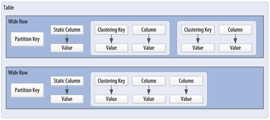
#### HBase Data Model
HBase stores data as a sparse, multidimensional, sorted map.
The map is indexed by its key (the row key), and values are stored in cells (consisting of a column key and column value). The row key and column keys are strings and the column value is an uninterpreted byte array (which could represent any primitive or complex datatype).
HBase is multidimensional, as each cell is versioned with a time stamp.
Row columns are grouped into column families. At table design time, one or more column families is defined. Column families will be used as physical storage groups for columns. Different column families may have different physical storage characteristics such as block size, compression settings, or the number of cell versions to retain.
A table’s column families must be specified up front as part of the table schema definition, but new column family members can be added on demand.
Physically, all column family members are stored together on the file system. We can say HBase is a column-family-oriented store.

* **info:format** and **info:geo** are both members of the info column family
* **contents:image** belongs to the contents family.
* A new column **info:camera** can be offered by a client as part of an update
#### Regions
Tables are automatically partitioned horizontally by HBase into regions. Each region comprises a subset of a table’s rows, usually a range of sorted row keys.
Initially, a table comprises a single region, but as the region grows it eventually crosses a configurable size threshold, at which point it splits at a row boundary into two new regions of approximately equal size. Until this first split happens, all loading will be against the single server hosting the original region.
Regions are the units that get distributed over an HBase cluster.
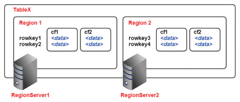
Like HDFS is built of clients, workers, and a coordinating master, the namenode and datanodes, HBase is made up of an HBase **master**node orchestrating a cluster of one or more **regionserver** workers.
The HBase master is responsible for assigning regions to registered regionservers, and for recovering regionserver failures.
The regionservers manage region splits, informing the HBase master about the new daughter regions so it can manage the offlining of parent regions and assignment.
### HBase browser in HUE
#### Add HBase Thrift Server role
The Thrift Server role is not added by default when you install HBase, but it is required before you can use certain other features such as the Hue HBase browser.
Follow the below steps to add the Thrift Server role:
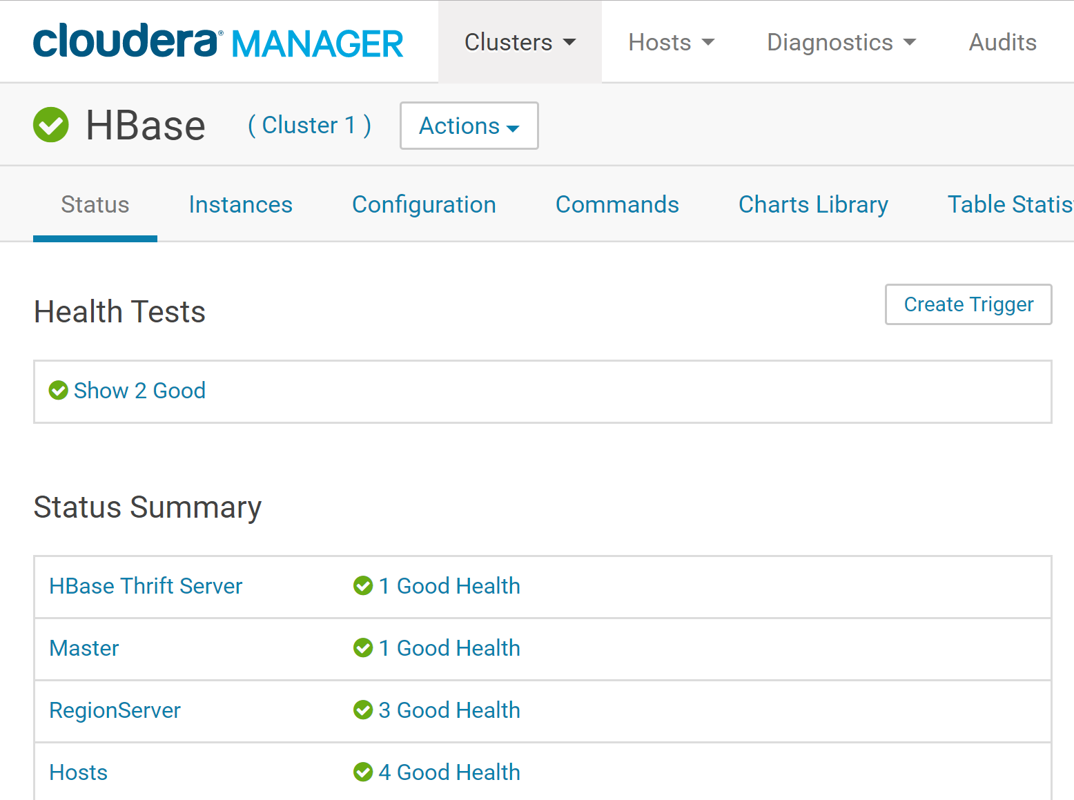
In Cloudera Manager, go to the HBase service:
Click the Instances tab.:
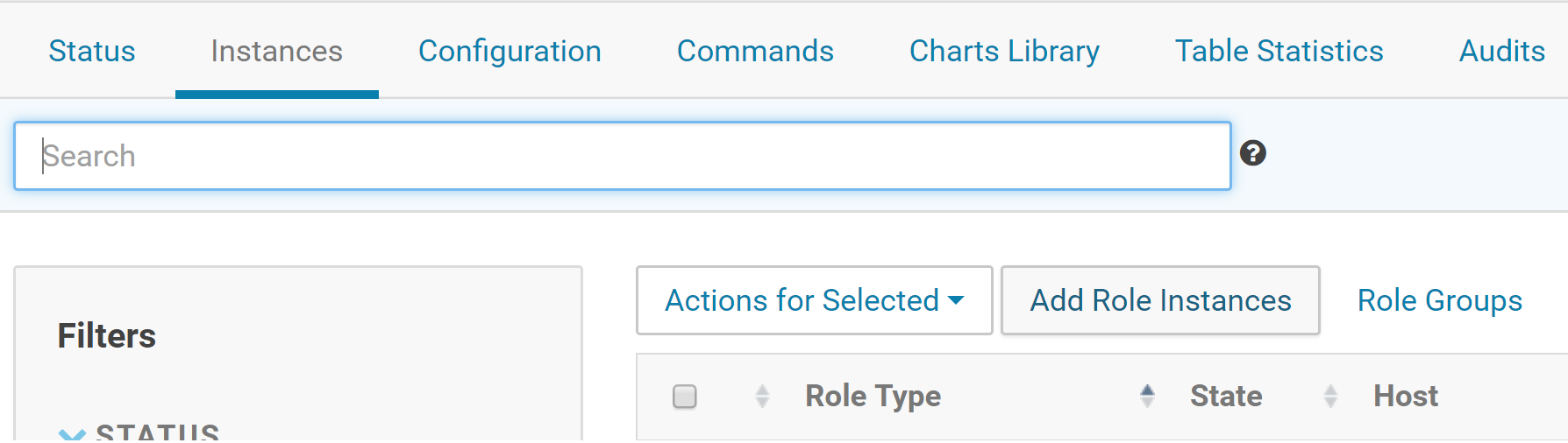
Click the Add Role Instances button.
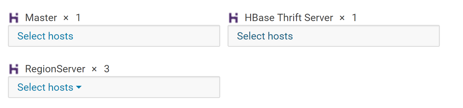
Select the host(s) where you want to add the Thrift Server role (you only need one for Hue) and click Continue. The Thrift Server role should appear in the instances list for the HBase server.

Select the Thrift Server role instance.
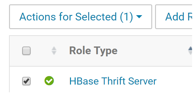
Select Actions for Selected > Start.
#### Configure Hue to point to the Thrift Server
In Cloudera Manager, select the Hue service.
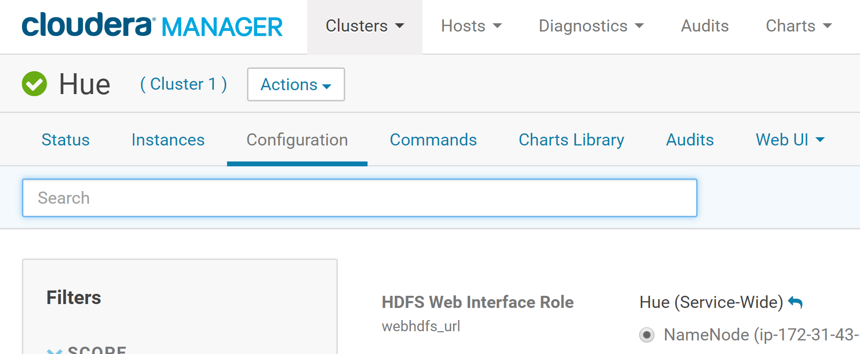
Click the Configuration tab.
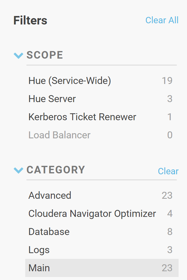
Select Scope > All.
Select Category > Main.
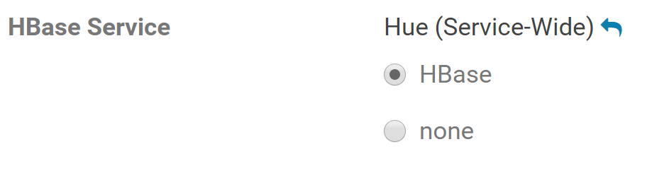
For the HBase Service property, make sure it is set to the HBase service for which you enabled the Thrift Server role (if you have more than one HBase service instance).
In the HBase Thrift Server property, click the edit field and select the Thrift Server role for Hue to use.

Select Category > Advanced.
Locate the Hue Service Advanced Configuration Snippet (Safety Valve) for hue\_safety\_valve.ini property and add the following property:
```
[hbase]
hbase_conf_dir=/etc/hbase/conf
```
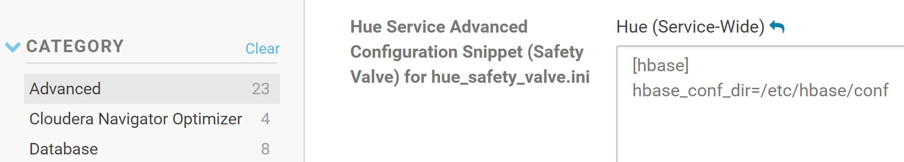
Click Save Changes to commit the changes.
### Demo HBase
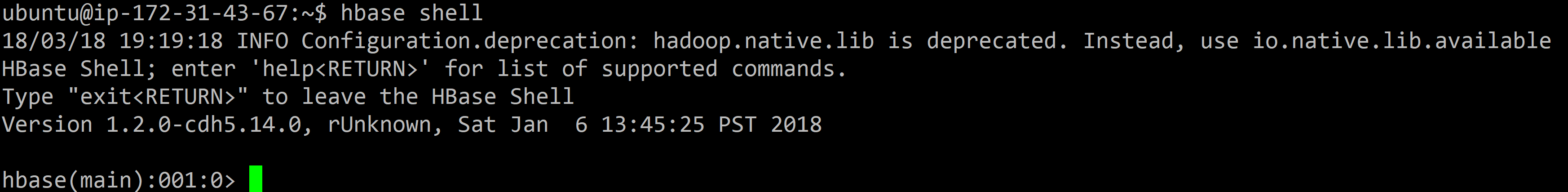
Connect to your cluster using SSH and run the HBase shell:
```
hbase shell
```
Create a new HBase table with two column families (cf1 and cf2) using the following statement:
```
create 'my-hbase-table', \
{NAME => 'cf1' , VERSIONS => 3}, \
{NAME => 'cf2'}
```
VERSIONS => 4 means we want to keep 4 versions maximum of this column.
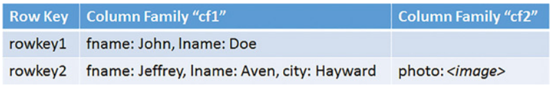
The subsequent put statements insert data into a cell as defined by the row key (**rowkey1** or **rowkey2**, in this case) and a column specified in the format **\:\**.
Unlike a traditional database, the columns are not defined at table design time and are not typed.
```
put 'my-hbase-table', 'rowkey1', 'cf1:fname', 'John'
put 'my-hbase-table', 'rowkey1', 'cf1:lname', 'Doe'
put 'my-hbase-table', 'rowkey2', 'cf1:fname', 'Jeffrey'
put 'my-hbase-table', 'rowkey2', 'cf1:lname', 'Aven'
put 'my-hbase-table', 'rowkey2', 'cf1:city', 'Hayward'
put 'my-hbase-table', 'rowkey2', 'cf2:photo', ''
```
Enter the scan command to show the content of the table:
```
scan 'my-hbase-table'
```

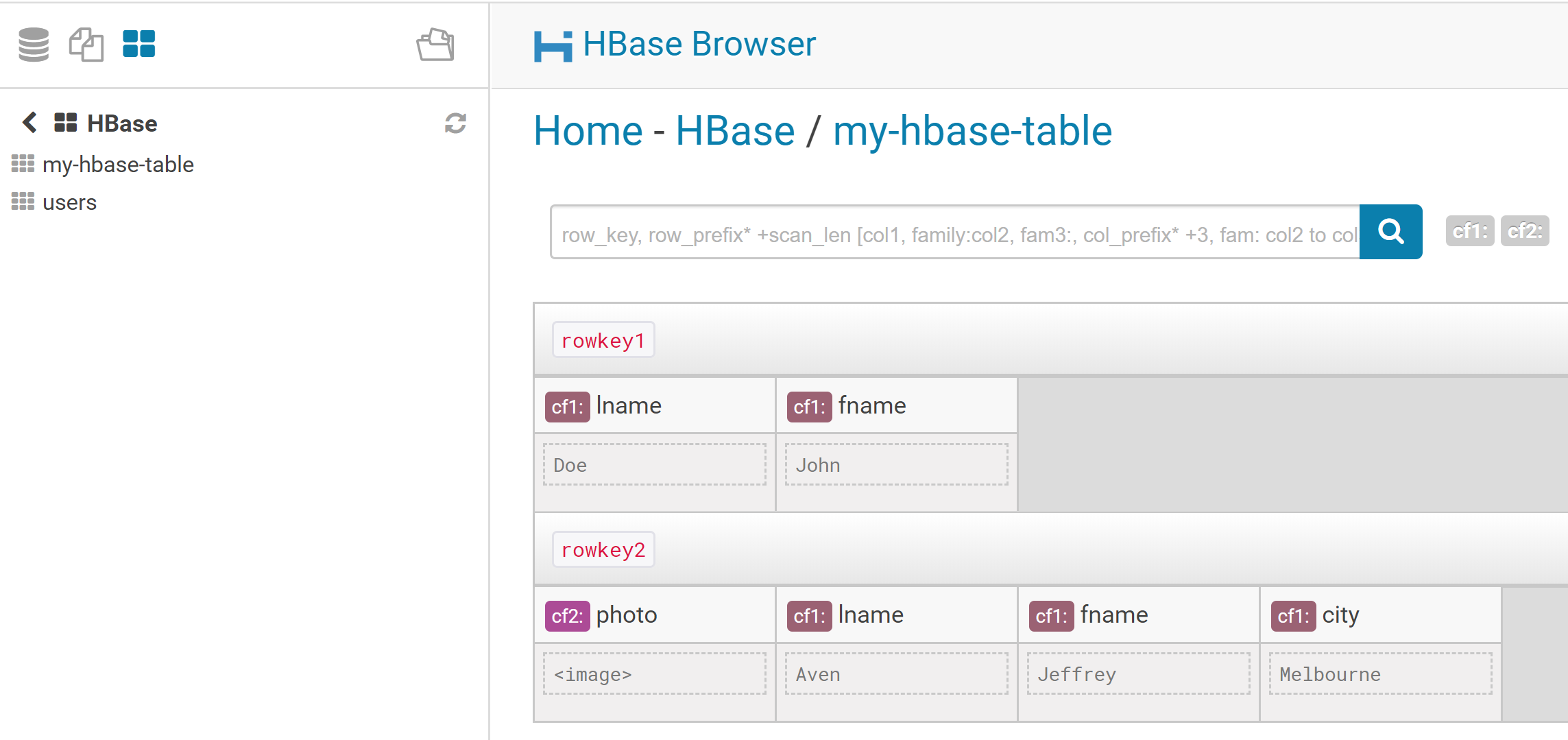
The data inserted you see in the console can be conceptually viewed like this:
HBase supports sparsity. Not every column needs to exist in each row in a table and nulls are not stored.
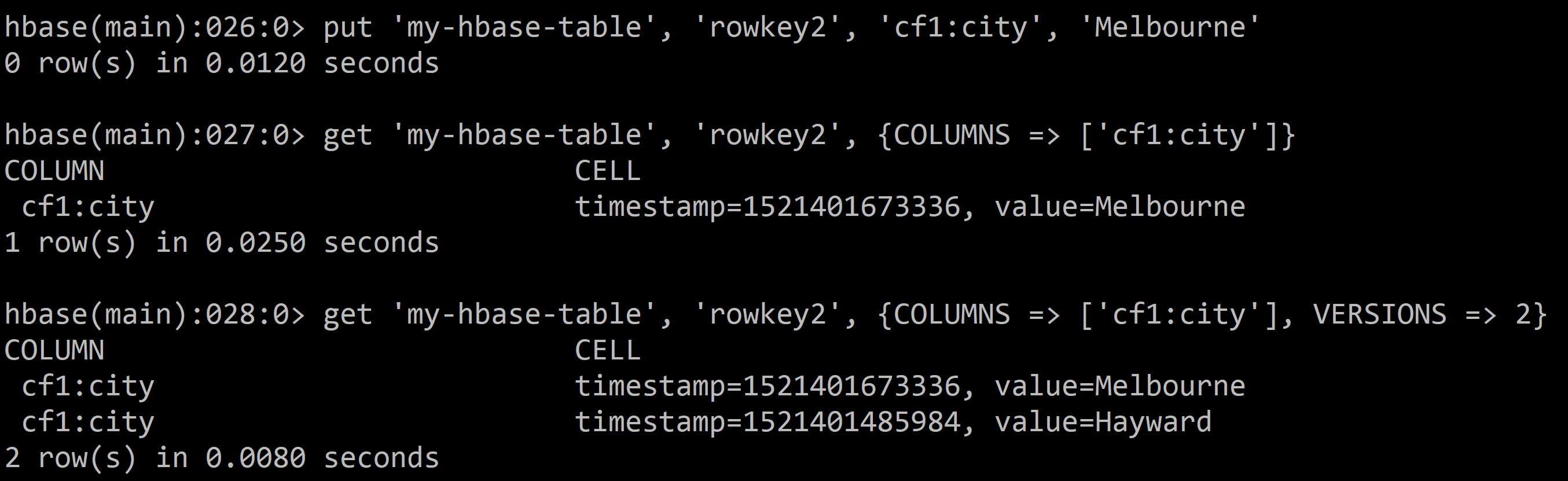
Although HBase data is stored on HDFS, an immutable file system, HBase allows in-place updates to cells within HBase tables. It does this by creating a new version of the cell with a new time stamp if the column key already exists, and then a background compaction process collapses multiple files into a smaller number of larger files.
Update a cell:
```
put 'my-hbase-table', 'rowkey2', 'cf1:city', 'Melbourne'
```
Get the latest version of a cell:
```
get 'my-hbase-table', 'rowkey2', {COLUMNS => ['cf1:city']}
```
Get multiple versions of a cell:
```
get 'my-hbase-table', 'rowkey2', {COLUMNS => ['cf1:city'], VERSIONS => 2}
```
Log in to HUE. The HBase browser should now be available in the main menu.
We can now browse across HBase tables using in HUE:
To drop the table in HBase, type-in the following command in the HBase shell (NOTE: you need to disable a table prior to dropping the table in HBase):
```
disable 'my-hbase-table'
drop 'my-hbase-table'
```
#### Load a file in HDFS into HBase using Pig
Suppose we have a file in HDFS we want to load into a HBase table. We can easily do that using Pig. This can be done in two steps:
1. Create the table in HBase.
2. Run the Pig script to load the file into the newly created table.
Let's consider we want to move the file **u.user** located in **/user/ubuntu/ml-100k/** to HBase. This file has 5 columns and is pipe (|) delimited.
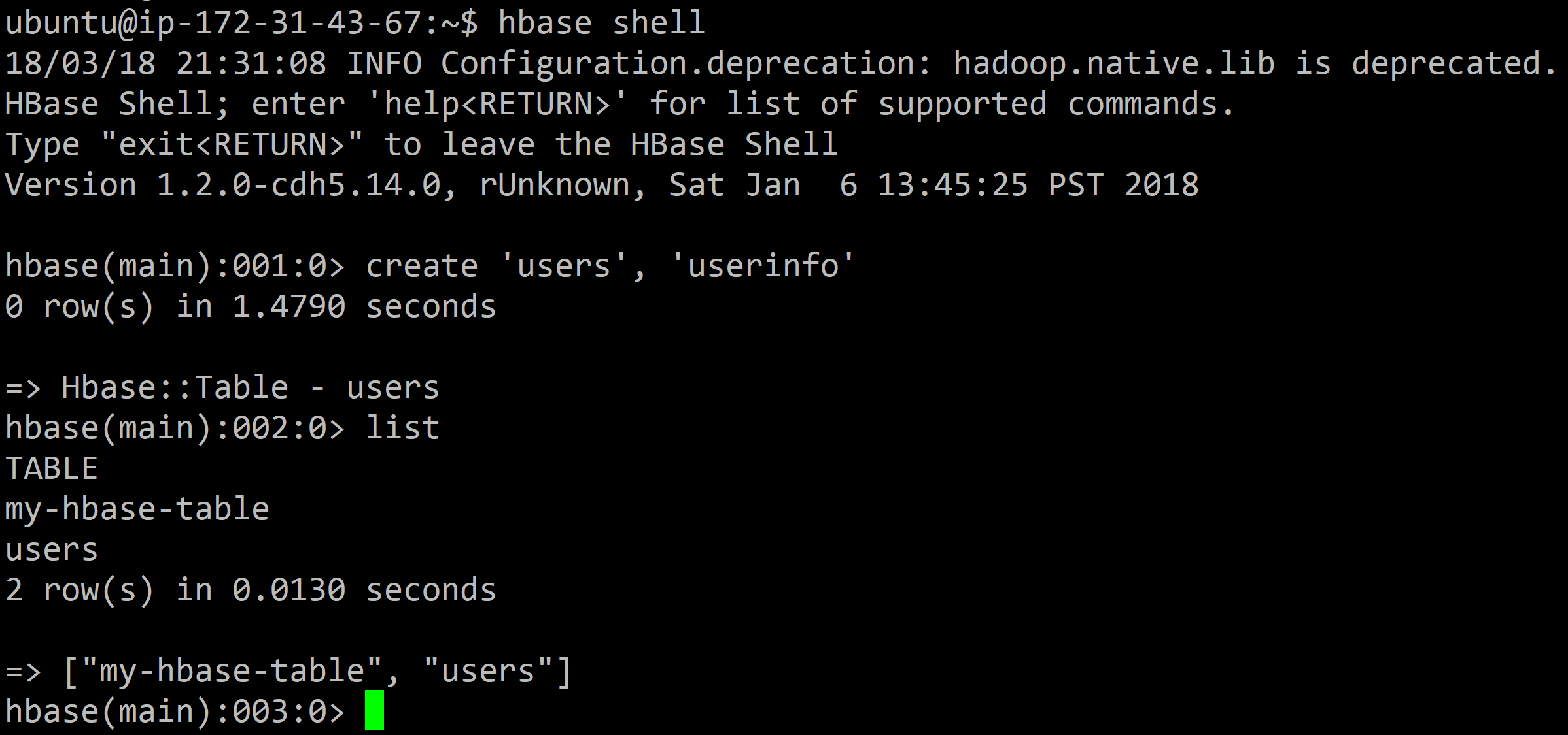
In the Terminal, enter the HBase shell:
```
hbase shell
```
Then create a new table **users** with one column family **userinfo** using the following command:
```
create 'users', 'userinfo'
```
Exit the HBase shell
```
exit
```
and run the Pig shell/Grunt:
```
pig
```
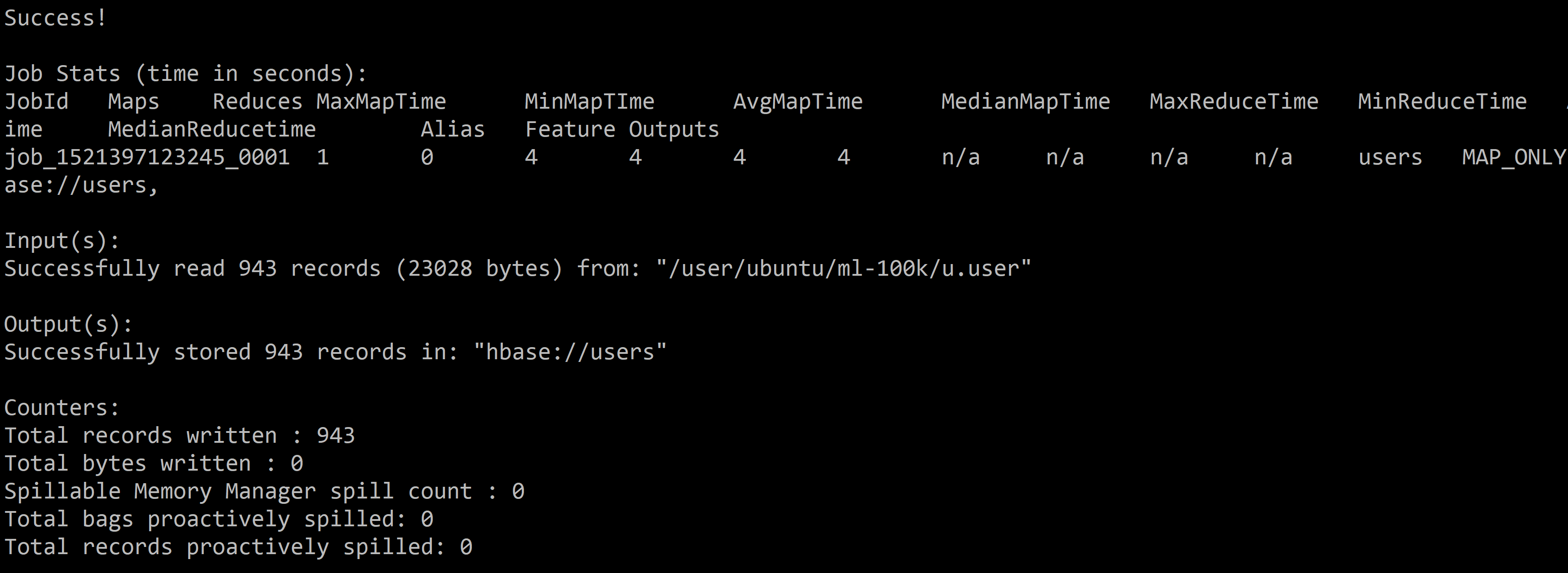
In the Pig shell, run the following command to load the file:
```
users = LOAD '/user/ubuntu/ml-100k/u.user'
USING PigStorage('|')
AS (userID:int, age:int, gender:chararray, occupation:chararray, zip:int);
```
Then we can store the relation in the HBase table. By default, the first column of the relation will be the row key of the HBase table.
```
STORE users INTO 'hbase://users'
USING org.apache.pig.backend.hadoop.hbase.HBaseStorage (
'userinfo:age,userinfo:gender,userinfo:occupation,userinfo:zip');
```
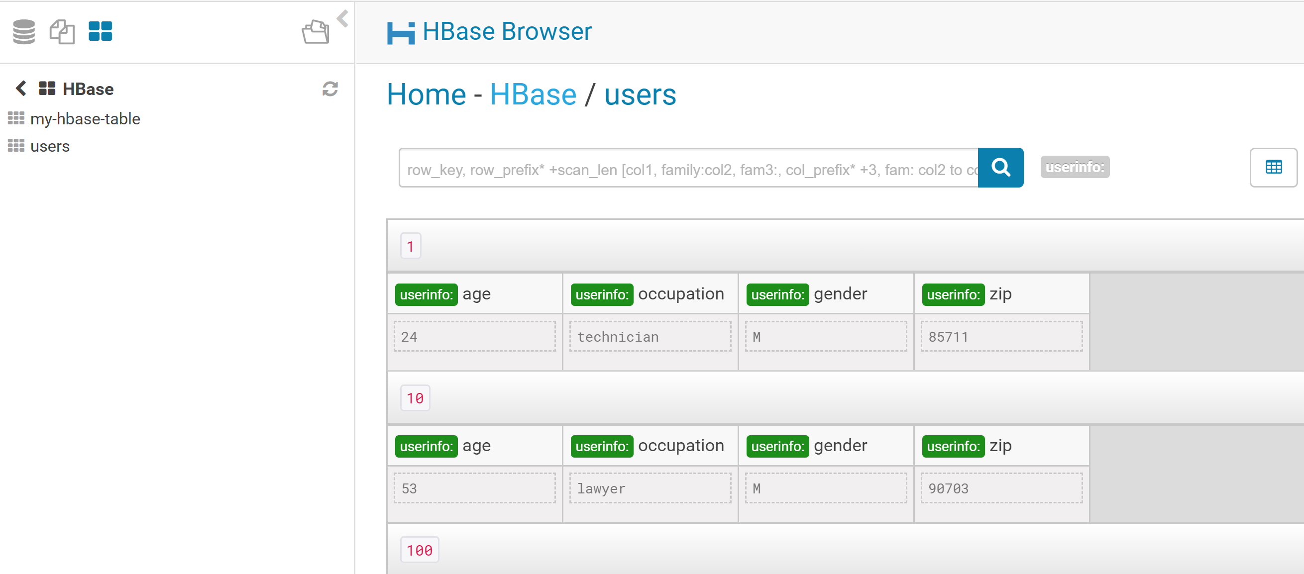
We can now browse the table in HUE using the HBase browser:
## Cassandra
Another notable project emanating from the Bigtable paper is Apache Cassandra.
Cassandra was initially developed at Facebook and later released as an open source project under the Apache software licensing scheme in 2008.
Cassandra became a top-level Apache project in 2010.
**Apache Cassandra is an open source, distributed, decentralized, elastically scalable, highly available, fault-tolerant, tuneably consistent, row-oriented database that bases its distribution design on Amazon’s Dynamo and its data model on Google’s Bigtable. Created at Facebook, it is now used at some of the most popular sites on the Web.**
#### Distributed and Decentralized
Cassandra is **distributed**, which means that it is capable of running on multiple machines while appearing to users as a unified whole.
Cassandra is **decentralized**, meaning that every node is identical; no Cassandra node performs certain organizing operations distinct from any other node.
The fact that Cassandra is decentralized means that there is **no single point of failure**.
All of the nodes in a Cassandra cluster function exactly the same as opposed to the **master/slave relationship** in HBase for example.
#### Elastic Scalability
**Scalability** is an architectural feature of a system that can continue serving a greater number of requests with little degradation in performance.
* **Vertical scaling** — simply adding more hardware capacity and memory to your existing machine — is the easiest way to achieve this.
* **Horizontal scaling** means adding more machines that have all or some of the data on them so that no one machine has to bear the entire burden of serving requests.
**Elastic scalability** refers to a special property of horizontal scalability. It means that your cluster can seamlessly scale up and scale back down.
Cassandra allows to easily add or remove machines or nodes as needed.
#### Tuneable Consistency
Consistency essentially means that a read always returns the most recently written value.
Cassandra trades some consistency in order to achieve total availability.
Cassandra is frequently called “**eventually consistent**”, which is a bit misleading.
Eventual consistency means on the surface that all updates will propagate throughout all of the replicas in a distributed system, but that this may take some time. Eventually, all replicas will be consistent.
Cassandra is more accurately termed “**tuneably consistent**”, which means it allows you to easily decide the level of consistency you require, in balance with the level of availability.
Tuneably consistency is achieved by controlling the number of replicas to block on for all updates.
This is done by setting the consistency level against the replication factor.
* The **replication factor** lets you decide how much you want to pay in performance to gain more consistency. You set the replication factor to the number of nodes in the cluster you want the updates to propagate to.
* The **consistency level** is a setting that clients must specify on every operation and that allows you to decide how many replicas in the cluster must acknowledge a write operation or respond to a read operation in order to be considered successful.
If the consistency level = replication factor -> we gain stronger consistency. At the cost of synchronous blocking operations that wait for all nodes to be updated and declare success before returning (impacts availability).
If consistency level < replication factor -> the update is considered successful even if some nodes are down.
#### Row-Oriented
Cassandra’s data model can be described as a partitioned row store, in which data is stored in sparse multidimensional hashtables. Cassandra has frequently been referred to as a “column-oriented” database. But Cassandra’s data store is not organized primarily around columns.
“**Sparse**” means that for any given row we can have one or more columns, but each row doesn’t need to have all the same columns as other rows like it (as in a relational model).
“**Partitioned**” means that each row has a unique key which makes its data accessible, and the keys are used to distribute the rows across multiple data stores.
### Cassandra Data Model
Cassandra uses a unique identifier/primary key for each row. Rows can be seen as a group of columns that should be treated together as a set.
We don’t need to store a value for every column every time we store a new entity. We have a sparse, multidimensional array structure.
Rows can be wide or skinny, depending on the number of columns the row contains.
A wide row is a row that has lots (perhaps tens of thousands or even millions) of columns. Typically there is a smaller number of rows that go along with so many columns.
Conversely, we can have a smaller number of columns and use many different rows, closer to the relational model. That’s the skinny model (as seen on the previous slide).
#### Wide Rows
Cassandra uses a special primary key called a **composite key** (or compound key) to represent **wide rows**, also called partitions.
The composite key consists of a **partition key**, plus an optional set of **clustering columns**.
The partition key is used to determine the nodes on which rows are stored.
The clustering columns are used to control how data is sorted for storage within a partition.
Cassandra also supports an additional construct called a static column, which is for storing data that is not part of the primary key but is shared by every row in a partition.
### Gossip protocol
To support decentralization and partition tolerance, Cassandra uses a **gossip protocol** that allows each node to keep track of state information about the other nodes in the cluster.
The gossiper runs every second on a timer.
Gossip protocols
* generally assume a faulty network.
* are commonly employed in very large, decentralized network systems.
* are often used as an automatic mechanism for replication in distributed databases.
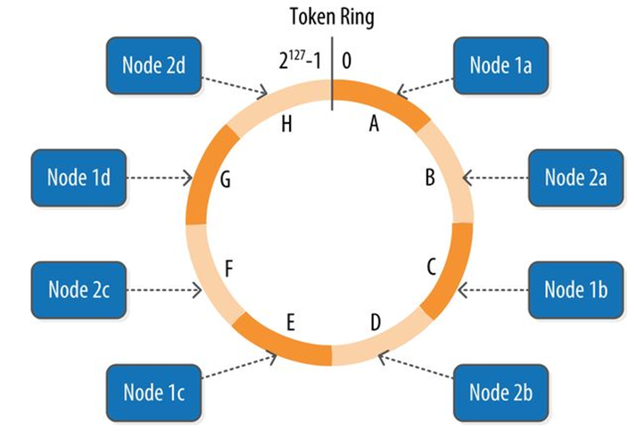
### Rings and Tokens
Cassandra keeps track of the physical layout of nodes in a cluster.
Cassandra represents the data managed by a cluster as a **ring**.
Each node in the ring is assigned one or more ranges of data described by a **token**, which determines its position in the ring.
A token is a 64-bit integer ID used to identify each partition.
Data is assigned to nodes by using a hash function to calculate a token for the partition key.
The partition key token is compared to the token values for the various nodes to identify the range, and therefore the node, that owns the data.
## MongoDB
MongoDB is a **document-oriented** database,
A document-oriented database replaces the concept of a “row” with a more flexible model, the “document.”
By allowing embedded documents and arrays, the document-oriented approach makes it possible to represent **complex hierarchical relationships** with a single record.
There are also **no predefined schemas**: a document’s keys and values are not of fixed types or sizes.
MongoDB’s document-oriented data model makes it easier for it to split up data across multiple servers (scaling out).
MongoDB automatically takes care of balancing data and load across a cluster, redistributing documents automatically and routing user requests to the correct machines.
Some features common to relational databases are not present in MongoDB, notably joins and complex multirow transactions.
A **document** is the basic unit of data for MongoDB and is roughly equivalent to a row in a relational database management system.
A **collection** can be thought of as a table with a **dynamic schema**. This means that the documents within a single collection can have any number of different “shapes.”
A single instance of MongoDB can host multiple independent databases, each of which can have its own collections.
Every document has a special key, "\_id", that is **unique within a collection**.
MongoDB comes with a simple but powerful **JavaScript shell**, which is useful for the administration of MongoDB instances and data manipulation.
Documents are an ordered set of keys with associated values. Most documents will contain multiple key/ value pairs. The keys in a document are strings.

### Replica Sets
Replication is a way of keeping identical copies of your data on multiple servers.
With MongoDB, you set up replication by creating a replica set.
A replica set is a group of servers with one primary, the server taking client requests, and multiple secondaries, servers that keep copies of the primary’s data.
If the primary crashes, the secondaries can elect a new primary from amongst themselves.

#### Replica Sets Quirks
A majority of the servers in your set must agree on the primary. Even numbers of servers (like 2) don’t work well.
If you have only 2 servers, you can set an **arbiter**, whose only purpose is to participate in elections. Arbiters hold no data and aren’t used by clients: they just provide a majority for two-member sets.
Replicas only address durability, not your ability to scale You can take advantage of reading from secondaries but this is generally not recommended. The database will still go into read-only mode for a bit while a new primary is elected (remember Availability in the CAP theorem).
### Sharding
**Sharding** refers to the process of splitting data up across machines; the term **partitioning** is also sometimes used to describe this concept.
MongoDB supports **autosharding**, which tries to both abstract the architecture away from the application and simplify the administration of such a system.
**Shards** store the data. Each shard is a replica set.
**Query Routers**, or mongos instances, interface with client applications and direct operations to the appropriate shard or shards.
**Config servers** store the cluster’s metadata. This data contains a mapping of the cluster’s data set to the shards.

---
# Agent Instructions
This documentation is published with GitBook. GitBook is the documentation platform designed so that both humans and AI agents can read, navigate, and reason over technical content effectively. Learn more at gitbook.com.
## Querying This Documentation
If you need additional information that is not directly available in this page, you can query the documentation dynamically by asking a question.
Perform an HTTP GET request on the current page URL with the `ask` query parameter:
```
GET https://jheck.gitbook.io/hadoop/data-storage.md?ask=
```
The question should be specific, self-contained, and written in natural language.
The response will contain a direct answer to the question and relevant excerpts and sources from the documentation.
Use this mechanism when the answer is not explicitly present in the current page, you need clarification or additional context, or you want to retrieve related documentation sections.